Example for using the Pvlib model

The Pvlib model can be used to determine the feed-in of a photovoltaic module using the pvlib. The pvlib is a python library for simulating the performance of photovoltaic energy systems. For more information check out the documentation of the pvlib.

The following example shows you how to use the Pvlib model.

• Set up Photovoltaic object
• Get weather data
• Calculate feed-in

Set up Photovoltaic object

To calculate the feed-in using the Pvlib model you have to set up a Photovoltaic object. You can import it as follows:

from feedinlib import Photovoltaic

To set up a Photovoltaic system you have to provide all PV system parameters required by the PVlib model. The required parameters can be looked up in the model’s documentation. For the Pvlib model these are the azimuth and tilt of the module as well as the albedo or surface type. Furthermore, the name of the module and inverter are needed to obtain technical parameters from the provided module and inverter databases. For an overview of the provided modules and inverters you can use the function get_power_plant_data().

from feedinlib import get_power_plant_data

# get modules
module_df = get_power_plant_data(dataset='sandiamod')
# print the first four modules
module_df.iloc[:, 1:5]

	Advent_Solar_Ventura_210___2008_	Advent_Solar_Ventura_215___2009_	Aleo_S03_160__2007__E__	Aleo_S03_165__2007__E__
Vintage	2008	2009	2007 (E)	2007 (E)
Area	1.646	1.646	1.28	1.28
Material	mc-Si	mc-Si	c-Si	c-Si
Cells_in_Series	60	60	72	72
Parallel_Strings	1	1	1	1
Isco	8.34	8.49	5.1	5.2
Voco	35.31	35.92	43.5	43.6
Impo	7.49	7.74	4.55	4.65
Vmpo	27.61	27.92	35.6	35.8
Aisc	0.00077	0.00082	0.0003	0.0003
Aimp	-0.00015	-0.00013	-0.00025	-0.00025
C0	0.937	1.015	0.99	0.99
C1	0.063	-0.015	0.01	0.01
Bvoco	-0.133	-0.135	-0.152	-0.152
Mbvoc	0	0	0	0
Bvmpo	-0.135	-0.136	-0.158	-0.158
Mbvmp	0	0	0	0
N	1.495	1.373	1.25	1.25
C2	0.0182	0.0036	-0.15	-0.15
C3	-10.758	-7.2509	-8.96	-8.96
A0	0.9067	0.9323	0.938	0.938
A1	0.09573	0.06526	0.05422	0.05422
A2	-0.0266	-0.01567	-0.009903	-0.009903
A3	0.00343	0.00193	0.0007297	0.0007297
A4	-0.0001794	-9.81e-05	-1.907e-05	-1.907e-05
B0	1	1	1	1
B1	-0.002438	-0.002438	-0.002438	-0.002438
B2	0.00031	0.00031	0.0003103	0.0003103
B3	-1.246e-05	-1.246e-05	-1.246e-05	-1.246e-05
B4	2.11e-07	2.11e-07	2.11e-07	2.11e-07
B5	-1.36e-09	-1.36e-09	-1.36e-09	-1.36e-09
DTC	3	3	3	3
FD	1	1	1	1
A	-3.45	-3.47	-3.56	-3.56
B	-0.077	-0.087	-0.075	-0.075
C4	0.972	0.989	0.995	0.995
C5	0.028	0.012	0.005	0.005
IXO	8.25	8.49	5.04	5.14
IXXO	5.2	5.45	3.16	3.25
C6	1.067	1.137	1.15	1.15
C7	-0.067	-0.137	-0.15	-0.15
Notes	Source: Sandia National Laboratories Updated 9...	Source: Sandia National Laboratories Updated 9...	Source: Sandia National Laboratories Updated 9...	Source: Sandia National Laboratories Updated 9...

# get inverter data
inverter_df = get_power_plant_data(dataset='cecinverter')
# print the first four inverters
inverter_df.iloc[:, 1:5]

	ABB__MICRO_0_25_I_OUTD_US_208__208V__208V__CEC_2018_	ABB__MICRO_0_25_I_OUTD_US_240_240V__CEC_2014_	ABB__MICRO_0_25_I_OUTD_US_240__240V__240V__CEC_2018_	ABB__MICRO_0_3_I_OUTD_US_208_208V__CEC_2014_
Vac	208.000000	240.000000	240.000000	208.000000
Paco	250.000000	250.000000	250.000000	300.000000
Pdco	259.589000	259.552697	259.492000	311.714554
Vdco	40.000000	39.982246	40.000000	40.227111
Pso	2.089610	1.931194	2.240410	1.971053
C0	-0.000041	-0.000027	-0.000039	-0.000036
C1	-0.000091	-0.000158	-0.000132	-0.000256
C2	0.000494	0.001480	0.002418	-0.000833
C3	-0.013171	-0.034600	-0.014926	-0.039100
Pnt	0.020000	0.050000	0.050000	0.020000
Vdcmax	50.000000	65.000000	50.000000	65.000000
Idcmax	6.489710	10.000000	6.487300	10.000000
Mppt_low	30.000000	20.000000	30.000000	30.000000
Mppt_high	50.000000	50.000000	50.000000	50.000000

Now you can set up a PV system to calculate feed-in for, using for example the first module and converter in the databases:

system_data = {
    'module_name': 'Advent_Solar_Ventura_210___2008_',  # module name as in database
    'inverter_name': 'ABB__MICRO_0_25_I_OUTD_US_208__208V__208V__CEC_2018_',  # inverter name as in database
    'azimuth': 180,
    'tilt': 30,
    'albedo': 0.2}
pv_system = Photovoltaic(**system_data)

Optional power plant parameters

Besides the required PV system parameters you can provide optional parameters such as the number of modules per string, etc. Optional PV system parameters are specific to the used model and how to find out about the possible optional parameters is documented in the model’s feedin method under power_plant_parameters. In case of the Pvlib model see here.

system_data['modules_per_string'] = 2
pv_system_with_optional_parameters = Photovoltaic(**system_data)

Get weather data

Besides setting up your PV system you have to provide weather data the feed-in is calculated with. This example uses open_FRED weather data. For more information on the data and download see the load_open_fred_weather_data Notebook.

from feedinlib.db import Weather
from feedinlib.db import defaultdb
from shapely.geometry import Point

# specify latitude and longitude of PV system location
lat = 52.4
lon = 13.5
location = Point(lon, lat)

# download weather data for June 2017
open_FRED_weather_data = Weather(
    start='2017-06-01', stop='2017-07-01',
    locations=[location],
    variables="pvlib",
    **defaultdb())

# get weather data in pvlib format
weather_df = open_FRED_weather_data.df(location=location, lib="pvlib")

/home/birgit/virtualenvs/feedinlib/lib/python3.6/site-packages/pandas/core/sorting.py:257: FutureWarning: Converting timezone-aware DatetimeArray to timezone-naive ndarray with 'datetime64[ns]' dtype. In the future, this will return an ndarray with 'object' dtype where each element is a 'pandas.Timestamp' with the correct 'tz'.
        To accept the future behavior, pass 'dtype=object'.
        To keep the old behavior, pass 'dtype="datetime64[ns]"'.
  items = np.asanyarray(items)

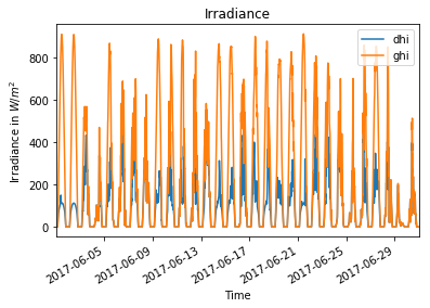
# plot irradiance
import matplotlib.pyplot as plt
%matplotlib inline
weather_df.loc[:, ['dhi', 'ghi']].plot(title='Irradiance')
plt.xlabel('Time')
plt.ylabel('Irradiance in $W/m^2$');

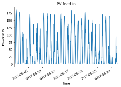
Calculate feed-in

The feed-in can be calculated by calling the Photovoltaic’s feedin method with the weather data. For the Pvlib model you also have to provide the location of the PV system.

feedin = pv_system.feedin(
    weather=weather_df,
    location=(lat, lon))

# plot calculated feed-in
import matplotlib.pyplot as plt
%matplotlib inline
feedin.plot(title='PV feed-in')
plt.xlabel('Time')
plt.ylabel('Power in W');

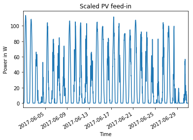
Scaled feed-in

The PV feed-in can also be automatically scaled by the PV system’s area or peak power. The following example shows how to scale feed-in by area.

feedin_scaled = pv_system.feedin(
    weather=weather_df,
    location=(lat, lon),
    scaling='area')

To scale by the peak power use scaling=peak_power.

The PV system area and peak power can be retrieved as follows:

pv_system.area

1.646

pv_system.peak_power

206.7989

# plot calculated feed-in
import matplotlib.pyplot as plt
%matplotlib inline
feedin_scaled.plot(title='Scaled PV feed-in')
plt.xlabel('Time')
plt.ylabel('Power in W');

Feed-in for PV system with optional parameters

In the following example the feed-in is calculated for the PV system with optional system parameters (with 2 modules per string, instead of 1, which is the default). It was chosen to demonstrate the importantance of choosing a suitable converter.

feedin_ac = pv_system_with_optional_parameters.feedin(
    weather=weather_df,
    location=(lat, lon))

# plot calculated feed-in
import matplotlib.pyplot as plt
%matplotlib inline
feedin_ac.plot(title='PV feed-in')
plt.xlabel('Time')
plt.ylabel('Power in W');

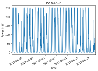
As the above plot shows the feed-in is cut off at 250 W. That is because it is limited by the inverter. So while the area is as expected two times greater as for the PV system without optional parameters, the peak power is only around 1.2 times higher.

pv_system_with_optional_parameters.peak_power / pv_system.peak_power

1.208903915833208

pv_system_with_optional_parameters.area / pv_system.area

2.0

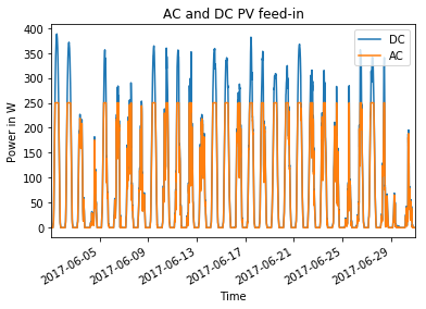
If you are only interested in the modules power output without the inverter losses you can have the Pvlib model return the DC feed-in. This is done as follows:

feedin_dc = pv_system_with_optional_parameters.feedin(
    weather=weather_df,
    location=(lat, lon),
    mode='dc')

# plot calculated feed-in
import matplotlib.pyplot as plt
%matplotlib inline
feedin_dc.plot(label='DC', title='AC and DC PV feed-in', legend=True)
feedin_ac.plot(label='AC', legend=True)
plt.xlabel('Time')
plt.ylabel('Power in W');

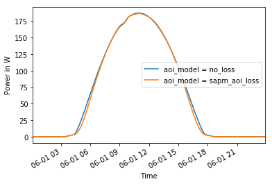
Feed-in with optional model parameters

In order to change the default calculation configurations of the Pvlib model to e.g. choose a different model to calculate losses or the solar position you can pass further parameters to the feedin method. An overview of which further parameters may be provided is documented under the feedin method’s kwargs.

feedin_no_loss = pv_system.feedin(
    weather=weather_df,
    location=(lat, lon),
    aoi_model='no_loss')

# plot calculated feed-in
import matplotlib.pyplot as plt
%matplotlib inline
feedin_no_loss.iloc[0:96].plot(label='aoi_model = no_loss', legend=True)
feedin.iloc[0:96].plot(label='aoi_model = sapm_aoi_loss', legend=True)
plt.xlabel('Time')
plt.ylabel('Power in W');